4.1 The Electromagnetic Field Equation
Scientists attempt to explain physical systems in terms of mathematical models which describe and predict the behavior of the system. For example, Kepler explained the movement of the planets with his three laws. In the same way, plasma behavior is governed by the electromagnetic field equations, which describe the motions of charged particles and their interaction with electric and magnetic fields. There are two components of the electromagnetic field equations: Maxwell’s Equations and the Lorentz Force Law. The two components act in tandem as a feedback loop:
Maxwell’s Equations determine the electric and magnetic fields based on the position and motion of charged particles. They also determine the interaction of the electric and magnetic fields if either is changing.
The Lorentz Force Law determines the electric and magnetic forces on a charged particle moving within the fields. This force will cause each particle to move (accelerate) in accordance with Newton’s Laws. The changes in the positions and motions of the charged particles in turn cause changes in the electric and magnetic fields.
Computer programs have been constructed to follow these interacting phenomena in plasmas. They typically involve a series of steps, each representing a very short span of time. First, given the state of magnetic and electric fields present and the mass, charge, speed and direction of each particle, using the Lorentz Force Law, the forces applied on each particle by the field values at its position (x,y,z coordinates) are calculated. The vector sum of the contributing forces is calculated, and the resulting acceleration of the particle moves it a small distance in some direction in the interval of the tiny time step (Newton’s Laws of Motion). This is accomplished for the entire set of particles.
Then, considering the new coordinates and kinematic conditions of each particle, Maxwell’s equations are used to determine the values of the electric and magnetic fields. After this, the program loops back to the first step, where the electric and magnetic forces acting on each particle are calculated once again using Lorentz Law.
The loop is controlled by the program’s directing it to stop when a defined condition is reached, such as a certain number of repetitions, or if a certain value in the variables is reached, changed, or exceeded, or an error of some kind is encountered, and so on.
Once a set of starting conditions has been defined (number of particles, their charges, masses, initial velocities, and a description of the intensities of the assumed electric and magnetic fields throughout a defined volume of space), the loop process above might be outlined as follows:
- Calculate all the forces acting on each particle via Lorentz Law
- Calculate new locations and velocities for a very short increment of time using Newton’s Laws of Motion
- Calculate E and B at each charged particle’s new location after this time increment
- If an End-Loop condition is not satisfied yet, go back to 1. and continue calculating
Other aspects can be added in for greater accuracy or a better approximation to “reality”, such as collisions of particles, viscous and gravity forces, etc. for more complete modeling. This is a complex undertaking, and large models with many particles may take months of supercomputer time to run.
This feedback loop can rapidly result in highly complex behavior, which is extremely difficult to model mathematically. Simplifications are often introduced. However, simplifying assumptions often lead to the omission of precisely those sorts of behavior which distinguish plasma behavior from that of a gas or other fluid.
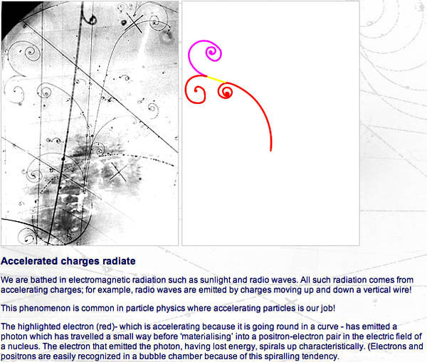
A bubble chamber within a magnetic field creates visible tracks of charged particles, allowing evaluation of particle energies, interactions and collision by-products, when installed in line with a particle accelerator. Image credit: Bubble chamber tutorial provided by CERN (link below)
Bubble chamber tutorial by CERN
A full description of the electromagnetic field equations can be found in Appendix II. What follows is a summary of the key points.
4.2 Maxwell’s Equations
The implications of Maxwell’s Equations and the underlying research are:
- A static electric field can exist in the absence of a magnetic field; e.g., a capacitor or a dust particle with a static charge Q has an electric field without a magnetic field.
- A constant magnetic field can exist without an electric field; e.g., a conductor with a constant current I has a magnetic field without an electric field.
- Where electric fields are time-variable, a nonzero magnetic field must exist.
- Where magnetic fields are time-variable, a nonzero electric field must exist.
- Magnetic fields can only be generated in two ways other than by permanent magnets: by an electric current, or by a changing electric field.
- Magnetic monopoles cannot exist; all lines of magnetic flux are closed loops.
4.3 The Lorentz Force Law
The Lorentz Force Law expresses the total force on a charged particle exposed to both electric and magnetic fields. The resultant force dictates the motion of the charged particle by Newtonian mechanics. As the Lorentz equation is fundamental to all plasma behavior, it is worth spending a little time understanding what it means. The equation is:
F = Q(E + U × B)
(Vectors are given in bold text and are explained below)
where F is the Lorentz force on the particle; Q is the charge on the particle; E is the electric field intensity; U is the velocity of the particle; B is the magnetic flux density, and “×” is the vector cross product symbol, not merely a multiplication sign. Read it as “U cross B”.
In order to understand what the equation actually means, we need to know a little about vectors.
A vector is a quantity which has both magnitude and direction. Examples include velocity and force. It is like an arrow: it has a length and it points in a direction. By contrast, a scalar quantity only has magnitude. Examples include speed and temperature. Vector algebra is the mathematics which deals with vectors. For those wanting to know, further details of vector algebra are given in Appendix III. The Hyperphysics explanation is also a good introduction. The essentials for understanding the Lorentz equation will be explained here.
First, multiplying a vector by a scalar quantity is like putting a number of similar arrows together end to end. The vector is the first arrow; the scalar quantity is the number of similar arrows. The result is a bigger arrow in the same direction as the original vector.
A simplified example is increasing the speed of a car to three times its initial speed as it moves in a straight line. Imagine that the car’s velocity vector is simply an arrow pointing straight ahead down the roadway, with its base or starting point always at the center of the car. Picture this arrow as being 20 cm long to represent a starting speed of 20 km/hour. Then you push down on the accelerator pedal to make the wheels of the car turn faster and push (accelerate) the car to a higher speed. As the car speeds up, the length of the arrow increases so that it always matches the car’s speed. At 60 km/hour the arrow is 60 cm long, and its direction is still parallel to the roadway. If you press the brake pedal, the car accelerates in the opposite direction, slowing down, and the arrow becomes shorter and shorter. As the car stops, its speed drops to zero, and the velocity arrow or vector becomes zero in length.
“That is easy to understand”, you say. “What happens if I turn the steering wheel to, say, the left?” That kind of an action introduces an additional force on the car, in a different direction from that pointing parallel to the centerline of the car. It does not increase or decrease its speed (neglecting friction!) but something changes because the car is turning! The velocity vector from the wheels making it go 60 km/hour has not changed length, but an additional force in a different direction has been applied, so now the velocity vector becomes the result of two different forces (two arrows acting on the center of the car). As long as you hold the steering wheel at the same angle, the same force is being applied that wants to turn the car, and it moves around on a circle at a constant speed.
You can see that there are two kinds of acceleration: changes in the speed of motion, either faster or slower – just a plain numerical value change in the distance per unit time ratio without reference to any direction – and changes to the direction of motion – just an angular change of the direction in space that something is heading, without reference to how fast along its path or trajectory it is moving. Both types of change are the result of a force being applied to an object.
Multiplying two vectors together is a little more complicated. Think of a very large screw in a wood board where the slot in the head represents the first vector and the second vector is drawn on the board. As the screw is twisted clockwise until the slot aligns with the second vector, the screw will move into the board at right angles to both the slot and the second vector. The amount of movement depends on the dimensions of the screw and the amount it is turned. The vector cross product is a bit like this.
Multiplying two vectors together using the cross product results in another vector at right angles to both the previous vectors – that is, perpendicular to the plane containing the two previous vectors. The direction of the new vector is given by the direction of movement of our imaginary screw. The magnitude (length) of the new vector depends both on the angle turned and on the size of the original vectors.

As in the case of our screw, if the vectors are aligned (parallel) in the first place, then no movement of the screw takes place. The cross product of aligned vectors is zero.
More formally, in Cartesian coordinates, if a vector in the x direction is crossed with a vector in the y direction, then the result is a vector in the z direction. The magnitude of the resultant vector is the triple product of the lengths of the two original vectors and the sine of the smaller angle between them. If they are parallel, the angle between them is zero. Since sine(0°) is zero, in that case there is no resultant force in the z direction.
The effect is very similar to the gyroscopic effect in rotating solids: a force in one direction results in motion in a direction at right angles. This is known as precession.
Going back to the Lorentz Force Law, we see that the total force is made up of two parts. The first part is QE, which is the product of the scalar value of the charge on the particle and the electric field strength vector. The magnitude of the force due to the electric field is the product of the charge on the particle and the strength of the electric field.
Note that the force due to the electric field is constant and in the direction of E, so it will cause constant acceleration of the particle in the direction of E according to Newton’s Laws of Motion, one direction for a positive charge, and the opposite direction for a negative charge.
The second part of the equation, Q(U × B) is more interesting. Here we have two vectors multiplied together using the cross product and then multiplied by the charge on the particle. Assuming that the particle was not moving in alignment with the field in the first place, when the force would be zero, then the result will be a force which is at right angles to both the direction of motion of the particle and the magnetic field. This explanation of the Right Hand Rule will explain the “steering” force that a magnetic field, in a specified direction, exerts on a charged particle entering the field.
A force at right angles to the motion is a centripetal force (definition: “toward the center”). The magnetic field will therefore cause the charged particle to move in a circle in a plane perpendicular to the direction of the magnetic field. As the particle is moving round the circle its velocity at any point will still have a component at right angles to the magnetic field, and so it will still experience a centripetal force which keeps it moving in the circle. Its direction is constantly changing, but its scalar speed (m/s) is unchanged, under this condition.
A simple case is to consider what happens when a moving charged particle enters a (fixed) magnetic field. For simplicity, we will ignore any effects that the particle might have upon the magnetic field. If it enters the field parallel to the direction of the field, it experiences no force and nothing about its velocity (scalar speed or direction) changes. If it enters the field at a right angle to the direction of the field, its path will simply curve into a circle which closes upon itself.
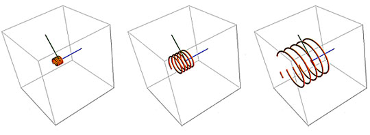
Without an electric field, the Lorentz law reads (centripetal force) F = Q(U × B). The force applied to the charged particle is directly proportional to Q, the particle’s charge, to U, the velocity vector, and to B, the magnetic field vector. The meaning of U × B is U times B times the sine of the smaller angle between the two vectors, which means that UB is multiplied by the sine of an angle, so its effect ranges from zero to 1. In the comparative illustration below, the particle’s charge and the magnetic field are held constant and the velocity of the particle as it enters the field increases from left to right. The faster the particle is moving, the larger the radius of the resultant circular motion, because the radius r is a measure of the particle’s linear momentum mU where m is the particle mass: r = mU ÷ (|Q|B). The same result would apply if the charge were to increase while the other two variables were held constant.
If the charged particle enters the magnetic field at an oblique angle, with a component of its motion vector in the direction of the field, i.e., at an angle between zero and 90 degrees to the field direction, it will “drift” in the direction parallel with the field, while the field forces the particle into a circular motion. This “drifting” circular path traces out a helix or spiral. The “guiding center” of the circle follows a field line of the magnetic field. The radius r is known as the Larmor radius or cyclotron radius. In the three illustrations below, the angle of entry by the particle and the strength of the magnetic field, B, remain the same, with a small drift motion toward the right. The initial entry velocity is increased step-wise from left to right, to show that the faster a charged particle enters a magnetic field, the larger its radius of curvature.
In the series of images below, the green entry vector touching the magnetic and electric field lines shows which way a positively charged particle (by convention) is moving as it “enters” the field(s). The particle could be going in either direction along this vector line at entry, so there are two trajectories coming out of the tip of the green vector, as you will see. If the particle were charged negatively, it would accelerate in the opposite direction, and if it were heavier or moving faster, it would have a larger diameter circle than depicted. Similarly, if the magnetic or electric fields were changed, holding other factors constant, that would similarly change the particle’s behavior. The narrow orange “tubes” represent the particle’s trajectory resulting from the entry conditions.
As a charged particle enters a uniform magnetic field B, its path is bent into a circle whose radius r is proportional to its linear momentum, mass times velocity (mU). The particle’s speed does not change, so its kinetic energy is unchanged, and the field does no work on the particle. This is analogous to gravity’s exerting a continuous centripetal force on an orbiting satellite in space. The magnetic field direction is shown by a blue axial line; particle entry angle by a green radial line.
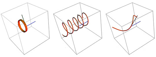
As the particle’s entry angle into the B-field changes from perpendicular to parallel, its trajectory will change to a spiral. The spiral will decrease in radius as the angle decreases from 90 degrees to the magnetic field direction and approaches zero or parallel to the field. Note the changing angle of the green entry vector, left to right, and the helical stretching. Images above created with Mathematica Demonstrations
The total force will be the vector resultant of the electric and magnetic forces and depends on the angle between the two fields (images below).
If the electric and magnetic fields are parallel (as in the field-aligned current situation we will consider later), then a charged particle approaching radially to the axial direction of the fields will be constrained to move in a helical path aligned with the direction of the fields. That is to say, the particle will accelerate (constantly change its direction to spiral around the axial direction of the magnetic field) as a result of the Lorentz force, and will simultaneously accelerate (change its scalar speed) in the direction of the electric field. This makes successive revolutions farther and farther apart as the particle’s velocity component in the E-field direction increases over time.
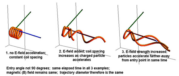
In this field-aligned situation (E and B fields parallel) a particle trajectory has the centripetal circularizing magnetic force applied at the same time that the E-field vector (red) forces it to accelerate axially. Over time the particle is moving nearly parallel to the fields.
If the charged particle enters the combined, aligned field axially (parallel to the magnetic field), it experiences no magnetic field, so force to revolve around a guiding center is not exerted. The electric field, however, will still accelerate the particle along the field lines. Depending on its charge, if the particle enters in the direction of the accelerating force, its velocity increases. If it enters counter to this force, it decelerates and may stop and accelerate back in the opposite direction. Recall that the “direction” of an electric field is defined as the direction that its force is applied to a positively-charged particle.
If the fields are not aligned, various trajectory combinations can occur depending on the particulars of the charge, field strengths, entry direction and angular misalignment of the magnetic and electric fields.
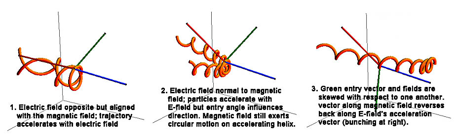
With a constant electric field present, its general tendency will be to accelerate particles ever more closely aligned with its field lines, and to increasing velocities. Images above created with Mathematica Demonstrations
Although these trajectories may look complex, they involve only a single charged particle at a time, with constant electric and magnetic fields, with the same entry velocity. In practice many charged particles of different polarities and velocity vectors may occupy a volume of space at once, and their electric and magnetic interactions will affect the field values in which they move.
There may also be neutral particles present, as well as dust and grains and large bodies, all of which may exert other forces (gravity, viscous, collisions) on the plasma interactions, too.

field-aligned relativistic electron producing X-ray wavelength synchrotron radiation
We note in passing that secondary effects of relativistic electrons spiraling around magnetic field lines in space are often detected in the form of synchrotron radiation. From consideration of the Lorentz Force Law, we know that there must therefore be an electric field aligned with the magnetic field and that the axial movement of the spiraling electrons with a velocity component parallel to the magnetic field constitutes a field-aligned current. These currents are Birkeland currents; they occur at many cosmic scales.
4.4 Other Effects of the Field Equations
It is worth remembering some basic results arising from the application of the electromagnetic field equations.
- Electric fields cause a force on all charged particles.
- The electric force will be in opposite directions for oppositely charged particles; therefore, an electric field will produce opposite velocities of ions and electrons and so tend to separate them. Charge separation in space is important in plasma physics.
- Magnetic fields only act on moving charged particles having a component of motion perpendicular to the magnetic field. Because the force depends on the cross-product of the velocity and field vectors, the effect will be different in different directions. This results in a direction-dependent electrical resistance. Think of trying to swim straight across a river rather than with the water’s current.
- The direction of the magnetic force is momentum and charge-dependent; ions and electrons will therefore circle in opposite directions with different radii and periods of rotation.
- Bulk plasma moving across the direction of a magnetic field will cause a local electric field to develop which itself will cause new forces on the charged particles.
- Changes in the distribution of charged particles cause a change in the electric field between them; a changing electric field generates a change in the magnetic field.
- The Maxwell Equations and the Lorentz Force Law act together as a feedback loop modifying the motions of the charged particles and the fields in complex ways.
4.5 Replacing Currents With Magnetic Fields
The question arises as to whether electric currents can be replaced by magnetic fields using Maxwell’s Equations, which would make the solutions much easier.
The answer is, technically, yes they can in certain simple situations, and this is often done in magneto-hydrodynamic theories and models because it is more convenient for studying certain plasma phenomena. However, there are many aspects of plasma behavior where it is necessary and crucial to consider the movement of the charged particles because simply considering the field behavior cannot model the observed complexity of plasma behavior.
The situation is analogous to the wave-particle duality in particle physics: there are some situations where it is necessary to use the particle description.
Examples of plasma behavior requiring use of the particle or current description include cellularization and filamentation, energy transport, and instabilities. Consideration of electric currents and circuits also necessitates the use of a particle-based description.
Simply considering only the field effects in these situations will miss the true complexity of plasma behavior. We shall look at some of these more complex behaviors next.

Galaxy Centaurus A as seen by Chandra in X-ray “light”, with central plasma jet and resultant plume structures spanning tens of thousands of light years
End of Chapter 4